Using ANN To Predict Euthanasia in LMAS Intake
Overview and Introduction
Driven by the desire to do something as fun and interesting as this post by the folks at Decision Science, I decided to dust off some previous work done on Louisville Metro Animal Services Animal [“LMAS”] Intake and Outcome data (you can get it here). The problems are sort of the same at the core - while the linked work focuses on customer churn, this analysis will focus on what information tends to predict a given animal will be euthanized at LMAS using Artificial Neural Networks (“ANN”).
This is also somewhat personal for me. Over the past year, our family has gone from four wonderful animals down to just one - and we are strongly considering adopting a new family member as a companion to our two kids. If I can identify an at-risk animal at LMAS, then I would love to rescue that animal ASAP. So - this is a fun project with hopefully a happy ending!
Before we jump into the data, let’s take a look at what tools we are loading in and our source for the data itself:
## Load Packages

# Data manipulation and pre-processing
library(tidyverse)
library(magrittr)
library(tidyquant)
library(recipes)
library(rsample)

# Data modeling
library(keras)
library(lime)
library(yardstick)
library(corrr)
library(forcats)

# Data visualization
library(ggiraph)
library(formattable)
library(DT)

## Read in Data

# Read in LMAS data
lmas_data_raw <- read_csv("https://data.louisvilleky.gov/sites/default/files/Animal_IO_Data_1.csv")
Now, let’s take a look at the data. The file contains roughly 20 columns of information of every animal that has come through the doors of LMAS since the early 2000s through this year. We have everything from the traditional cats and dogs all the way to the less-than-traditional livestock and rodents. In total, there are 150,002 rows of data here - meaning over that timeframe, that many animals have been brought into the LMAS system.
Of those that have come in, 69,599 have been euthanized through the years. The goal of this work is to figure out why - and try and keep it from happening at least one more time.
# Take a glimpse at the data
glimpse(lmas_data_raw)
## Observations: 150,002
## Variables: 22
## $ AnimalID <chr> "A460117", "A413916", "A387595", "...
## $ AnimalType <chr> "CAT", "DOG", "DOG", "DOG", "CAT",...
## $ IntakeDate <dttm> 2012-04-06 17:48:00, 2010-06-16 1...
## $ IntakeType <chr> "OWNER SUR", "STRAY", "STRAY", "ST...
## $ IntakeSubtype <chr> "EUTH REQ", "OTC", "OTC", "FIELD",...
## $ PrimaryColor <chr> "BLACK", "BROWN", "BROWN", "BROWN"...
## $ PrimaryBreed <chr> "DOMESTIC SHORTHAIR", "CHOW CHOW",...
## $ SecondaryBreed <chr> NA, "ROTTWEILER", "MIX", "MIX", NA...
## $ Gender <chr> "SPAYED FEMALE", "FEMALE", "FEMALE...
## $ SecondaryColor <chr> "WHITE", "BLACK", NA, "BLACK", "WH...
## $ DOB <dttm> 2002-04-06, 2010-04-16, NA, 1998-...
## $ IntakeReason <chr> NA, NA, NA, NA, NA, NA, NA, NA, NA...
## $ IntakeInternalStatus <chr> "AGED", "SICK", "EMACIATED", "EMAC...
## $ IntakeAsilomarStatus <chr> "TREATABLE/MANAGEABLE", "HEALTHY",...
## $ ReproductiveStatusAtIntake <chr> "ALTERED", "FERTILE", "FERTILE", "...
## $ OutcomeDate <dttm> 2012-04-06 20:16:00, 2010-06-22 1...
## $ OutcomeType <chr> "EUTH", "EUTH", "EUTH", "RTO", "EU...
## $ OutcomeSubtype <chr> "REQUESTED", "CONTAG DIS", "TIME/S...
## $ OutcomeReason <chr> NA, NA, NA, NA, NA, NA, NA, NA, NA...
## $ OutcomeInternalStatus <chr> "AGED", NA, NA, "EMACIATED", "AGGR...
## $ OutcomeAsilomarStatus <chr> "HEALTHY", "HEALTHY", "HEALTHY", "...
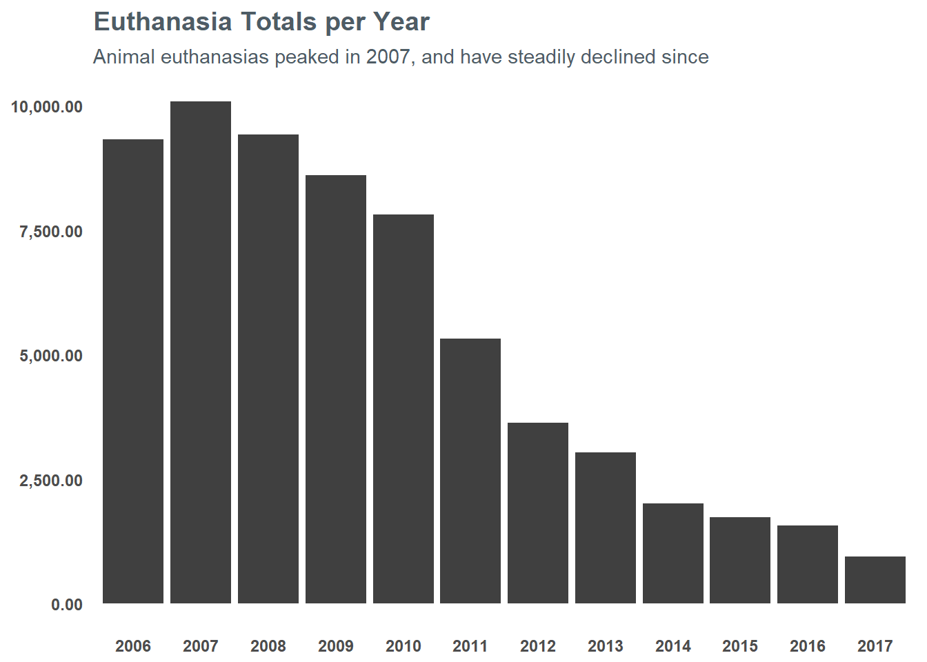
## $ ReproductiveStatusAtOutcome <chr> "ALTERED", "FERTILE", "FERTILE", "...I think it’s important to note that the trend of euthanasias has been going down for LMAS since the mid-2000s. In 2007, euthanasias peaked at just north of 10,000 and so far through 2017 they’re just south of 1,000 - which is just 10% of their peak a decade ago. You can see the steady decline in the chart below:
However, 1,000 a year is still quite a bit. In order to push that number even lower, we need to understand what the risk factors are for euthanasia for an animal. If we understand that, maybe we can help inform targeting resources to getting at-risk animals in front of folks. If nothing else, maybe I can help use it to direct my attention to adopting an animal with a high risk for euthanasia. So, let’s get started…
Feature Engineering and Data Pruning
There are a few fields that by themselves are not extremely interesting, but with a bit of feature design could be pretty informative:
DOBIntake DateOutcome Date
By themselves, these don’t tell us a whole lot. But using them, we can calculate an age (where DOB is provided) and length_of_stay (where known). This gives us the chance to use these as features in our final model. Once we have those ran, we can get rid of these as they are likely less informative than their derived features.
Additionally, it looks like there are a lot of NA values for some of the fields - too many to warrant dropping the rows completely while also not having enough non-NA values to use for imputing the missing data. For instance, 73% of Secondary Breed, 77% of Intake Reason, and 47% of Secondary Color. For Intake Reason I am actually going to keep those in because I am curious if having an unknown age is meaningful and if a known intake reason significantly sways the results, but for the other columns I am unfortunately going to need to remove them for the analysis.
## Feature Engineering
euth_data_tbl <- lmas_data_raw %>%
  # Remove intake where euthanasia was requested
  filter(!grepl("EUTH", IntakeReason),
         !grepl("EUTH", IntakeType),
         !grepl("EUTH", IntakeSubtype)) %>%
  # Reorder columns w/ OutcomeType upfront
  mutate(
    # Re-classify outcome type for euthanasia
    animal_euth = case_when(
      OutcomeType == "EUTH" ~ 1,
      TRUE ~ 0
    ),
    # Create age variable
    age = ((today() - ymd(DOB)) / 365) %>% as.integer(),
    # Calculate duration of length_of_stay
    length_of_stay = (ymd(as.Date(OutcomeDate)) - ymd(as.Date(IntakeDate))) %>% as.integer()) %>%
  # Remove columns
  select(
    # Remove unique outcome type (I've re-classified this)
    # Keep AnimalID to add back into table for reporting later
    -OutcomeType,
    # Remove feature engineered variables
    -IntakeDate,
    -DOB,
    -OutcomeDate,
    # Remove variables with too many NAs
    -SecondaryBreed,
    -SecondaryColor,
    # Remove variables relating to outcome
    -OutcomeSubtype,
    -OutcomeReason,
    -OutcomeInternalStatus,
    -OutcomeAsilomarStatus,
    -ReproductiveStatusAtOutcome) %>%
  # Reclassify NAs as -99 for age and unknown for intake reason and replace negative length_of_stay with 0
  mutate(
    age = case_when(
      is.na(age) ~ 0.01 %>% as.double(),
      age <=0 ~ 0.01 %>% as.double(),
      TRUE ~ age %>% as.double()
    ),
    IntakeReason = case_when(
      is.na(IntakeReason) ~ "unknown",
      TRUE ~ IntakeReason
    ),
    length_of_stay = case_when(
      length_of_stay < 0 ~ 0 %>% as.double(),
      TRUE ~ length_of_stay %>% as.double()
    )
  ) %>%
  # Move target to the first column
  select(animal_euth,
         everything()) %>%
  # Drop remaining NA rows
  drop_na()

# Take a glimpse of the euthanasia table
glimpse(euth_data_tbl)
## Observations: 138,810
## Variables: 14
## $ animal_euth <dbl> 1, 1, 0, 1, 1, 0, 1, 0, 0, 0, 0, 0,...
## $ AnimalID <chr> "A413916", "A387595", "A480549", "A...
## $ AnimalType <chr> "DOG", "DOG", "DOG", "CAT", "DOG", ...
## $ IntakeType <chr> "STRAY", "STRAY", "STRAY", "STRAY",...
## $ IntakeSubtype <chr> "OTC", "OTC", "FIELD", "FIELD", "FI...
## $ PrimaryColor <chr> "BROWN", "BROWN", "BROWN", "BLACK",...
## $ PrimaryBreed <chr> "CHOW CHOW", "GERMAN SHEPHERD DOG",...
## $ Gender <chr> "FEMALE", "FEMALE", "FEMALE", "FEMA...
## $ IntakeReason <chr> "unknown", "unknown", "unknown", "u...
## $ IntakeInternalStatus <chr> "SICK", "EMACIATED", "EMACIATED", "...
## $ IntakeAsilomarStatus <chr> "HEALTHY", "HEALTHY", "HEALTHY", "U...
## $ ReproductiveStatusAtIntake <chr> "FERTILE", "FERTILE", "FERTILE", "F...
## $ age <dbl> 7.00, 0.01, 19.00, 4.00, 0.01, 7.00...
## $ length_of_stay <dbl> 6, 18, 0, 11, 22, 8, 0, 9, 5, 9, 3,...Splitting the Data
The last step before transforming our data is to split it into two sets - a training set to use for building our model and a test set to apply the trained model to for performance measuring. To do this, we will just take a random sampling of our data and split 80% into training and the rest into testing.
# Set the seed for reproducibility
set.seed(1620)

# Create splits
splits <- initial_split(euth_data_tbl, prop = 0.8)

# Split data into train and test sets
euth_train_tbl <- training(splits)
euth_test_tbl  <- testing(splits)

# Save AnimalID for train and test (merge back in later)
animalID_train <- euth_train_tbl$AnimalID
animalID_test <- euth_test_tbl$AnimalID

# Remove animalID from train and test
euth_train_tbl$AnimalID <- NULL
euth_test_tbl$AnimalID <- NULL

glimpse(euth_train_tbl)
## Observations: 111,049
## Variables: 13
## $ animal_euth <dbl> 0, 1, 1, 0, 1, 0, 0, 0, 0, 1, 0, 0,...
## $ AnimalType <chr> "DOG", "CAT", "DOG", "CAT", "CAT", ...
## $ IntakeType <chr> "STRAY", "STRAY", "STRAY", "STRAY",...
## $ IntakeSubtype <chr> "FIELD", "FIELD", "FIELD", "OTC", "...
## $ PrimaryColor <chr> "BROWN", "BLACK", "BLACK", "CHOCOLA...
## $ PrimaryBreed <chr> "JACK RUSS TER", "DOMESTIC SHORTHAI...
## $ Gender <chr> "FEMALE", "FEMALE", "MALE", "NEUTER...
## $ IntakeReason <chr> "unknown", "unknown", "unknown", "u...
## $ IntakeInternalStatus <chr> "EMACIATED", "FERAL", "NORMAL", "NO...
## $ IntakeAsilomarStatus <chr> "HEALTHY", "UNHEALTHY/UNTREATABLE",...
## $ ReproductiveStatusAtIntake <chr> "FERTILE", "FERTILE", "FERTILE", "A...
## $ age <dbl> 19.00, 4.00, 0.01, 7.00, 3.00, 4.00...
## $ length_of_stay <dbl> 0, 11, 22, 8, 0, 5, 9, 3, 6, 3, 4, ...glimpse(euth_test_tbl)## Observations: 27,761
## Variables: 13
## $ animal_euth <dbl> 1, 1, 0, 1, 0, 0, 0, 1, 0, 1, 0, 1,...
## $ AnimalType <chr> "DOG", "DOG", "DOG", "DOG", "DOG", ...
## $ IntakeType <chr> "STRAY", "STRAY", "STRAY", "STRAY",...
## $ IntakeSubtype <chr> "OTC", "OTC", "FIELD", "FIELD", "FI...
## $ PrimaryColor <chr> "BROWN", "BROWN", "BUFF", "WHITE", ...
## $ PrimaryBreed <chr> "CHOW CHOW", "GERMAN SHEPHERD DOG",...
## $ Gender <chr> "FEMALE", "FEMALE", "MALE", "MALE",...
## $ IntakeReason <chr> "unknown", "unknown", "unknown", "u...
## $ IntakeInternalStatus <chr> "SICK", "EMACIATED", "NORMAL", "NOR...
## $ IntakeAsilomarStatus <chr> "HEALTHY", "HEALTHY", "HEALTHY", "H...
## $ ReproductiveStatusAtIntake <chr> "FERTILE", "FERTILE", "FERTILE", "F...
## $ age <dbl> 7.00, 0.01, 3.00, 5.00, 12.00, 5.00...
## $ length_of_stay <dbl> 6, 18, 9, 8, 11, 0, 0, 13, 10, 5, 4...Transforming the Data
Now that we have the data we want and engineered a few features, we need to transform for modeling. Certain variables will become individual dummy variables (the character stuff like Gender, AnimalType, etc.) but age and length_of_stay will likely need to be binned into groups for the sake of modeling.
Grouping data together
First, let’s focus on the numeric values and group them into appropriate values - starting with age. At first glance, there seems to be some skew in age - suggesting a log transformation may be best. When we do that, we can see that the distribution is slightly more normal from the logarithmic transformation - and testing a correlation suggests it might help the model in the end. So, based on that test we will run with the log transformation for our model.
# Plot count of age
euth_train_tbl %>%
  ggplot(aes(x = age)) +
  geom_histogram(fill = "#404040") +
  scale_y_continuous(labels = comma) +
  labs(title = "Count of Age",
       subtitle = "Ignoring the -99 values denoting 'unknown', age is fairly normally distributed")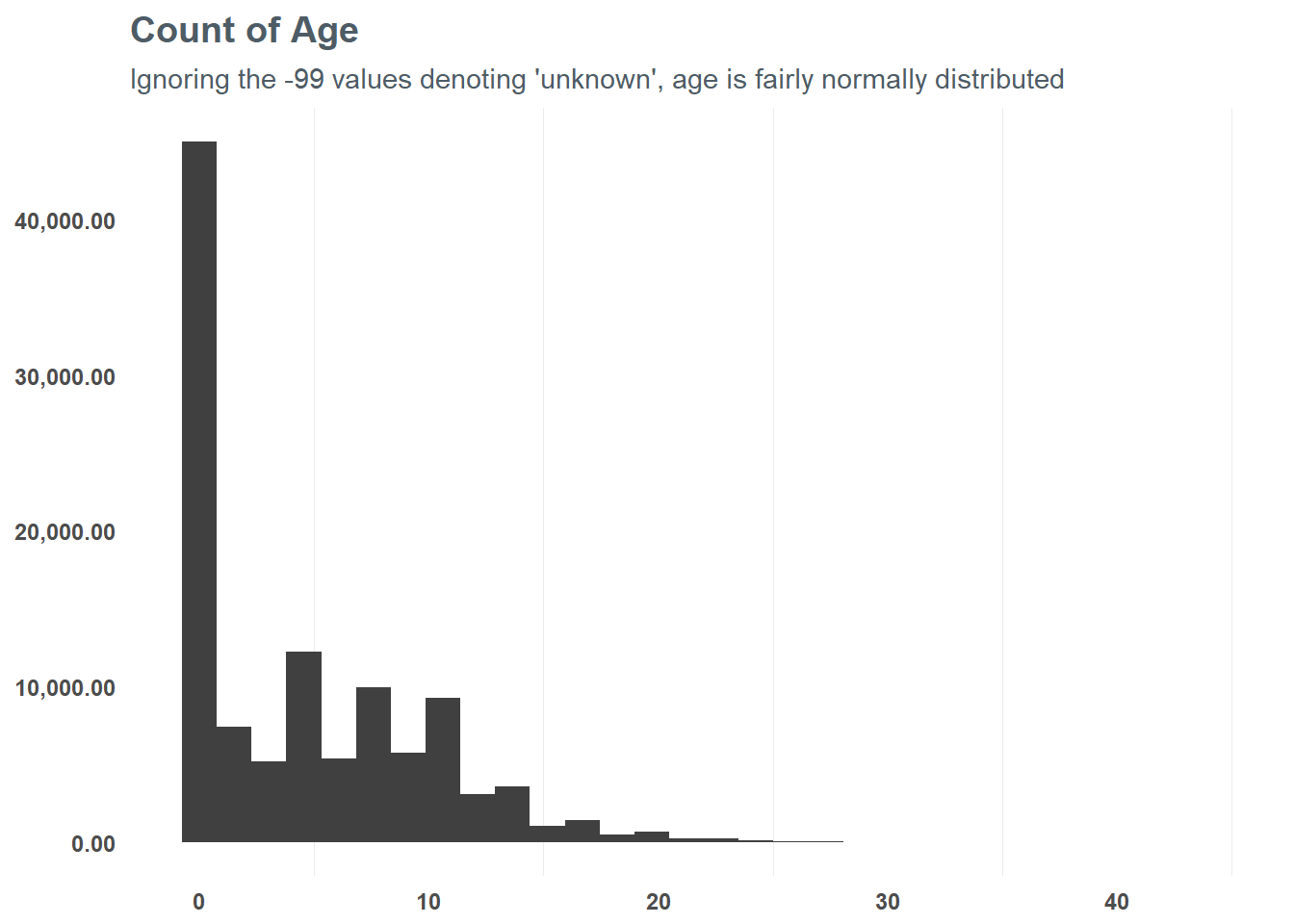
# We can do a better job of transforming the data
euth_train_tbl %>%
  ggplot(aes(x = log(age))) +
  geom_histogram(fill = "#404040") +
  scale_y_continuous(labels = comma) +
  labs(title = "Count of Age",
       subtitle = "Logging the age variable gives us a more normal distribution")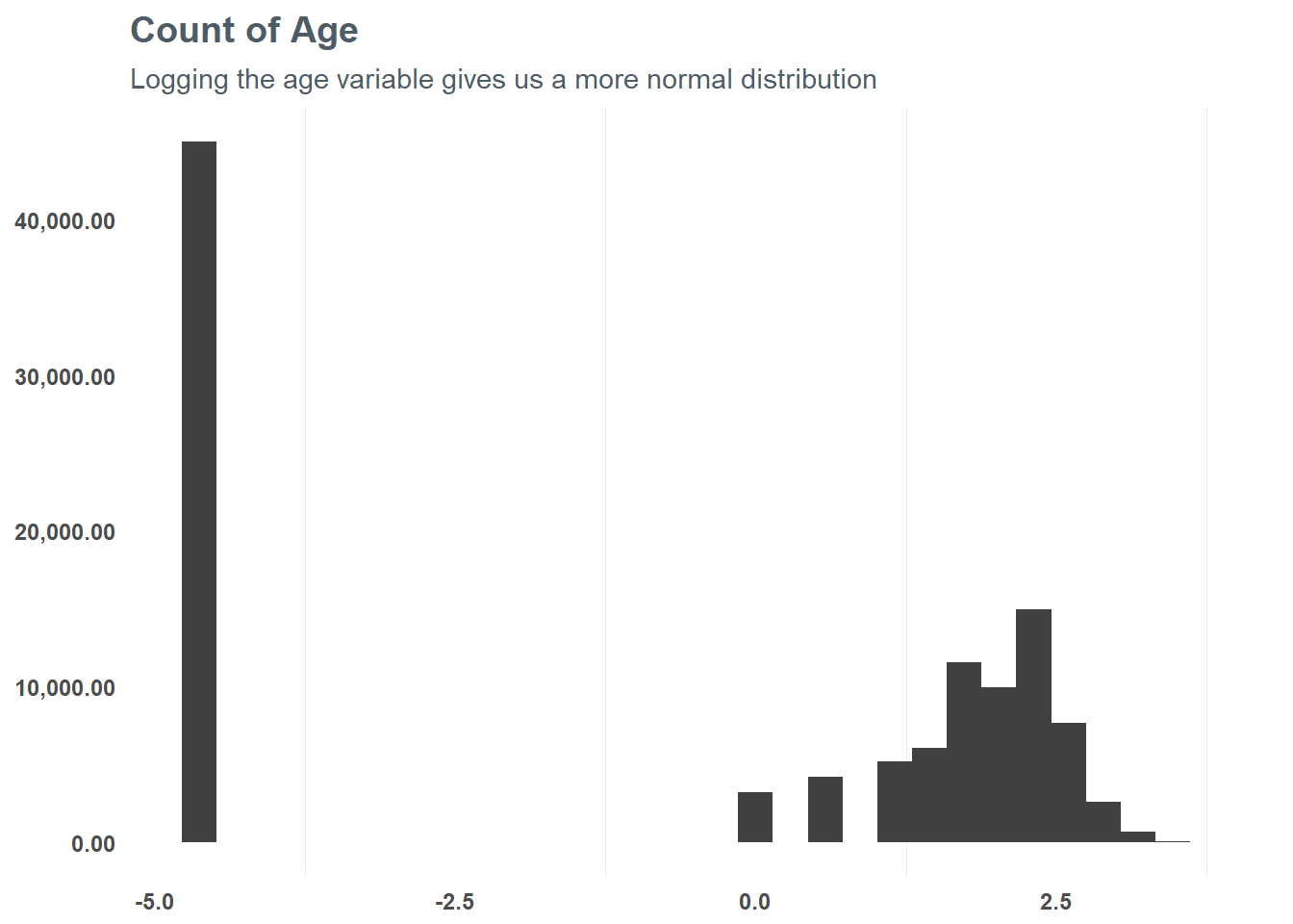
# Determine if log transformation improves correlation
euth_train_tbl %>%
    select(animal_euth, age) %>%
    mutate(
        logAge = log(age)
        ) %>%
    correlate() %>%
    focus(animal_euth) %>%
    fashion()
## rowname animal_euth
## 1 age -.19
## 2 logAge -.38Next, we want to take a look at length_of_stay. Unlike age, the length_of_stay variable is more uniformly distributed. BEcause of this, we can take advantage of grouping the variable into more distinct bins - letting us generalize the relationship of length_of_stay a bit more.
# Plot count of length_of_stay
euth_train_tbl %>%
  filter(length_of_stay <= 365) %>%
  group_by(length_of_stay) %>%
  summarise(total = n()) %>%
  ggplot(aes(x = length_of_stay)) +
  geom_histogram(fill = "#404040",
                 colour = "#ffffff") +
  scale_y_continuous(labels = comma) +
  labs(title = "Count of Length of Stay",
       subtitle = "The distribution of length of stay is far less skewed than age")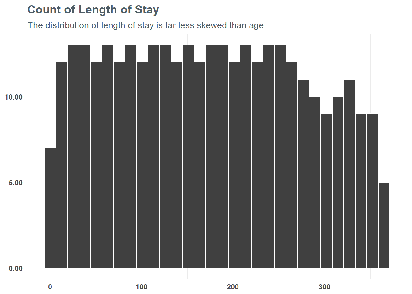
# Plot count of length_of_stay
euth_train_tbl %>%
  filter(length_of_stay <= 365) %>%
  group_by(length_of_stay) %>%
  summarise(total = n()) %>%
  ggplot(aes(x = length_of_stay)) +
  geom_histogram(bins = 5,
                 fill = "#404040",
                 colour = "#ffffff") +
  scale_y_continuous(labels = comma) +
  labs(title = "Count of Length of stay",
       subtitle = "Using bins of five to reduce variance within groups")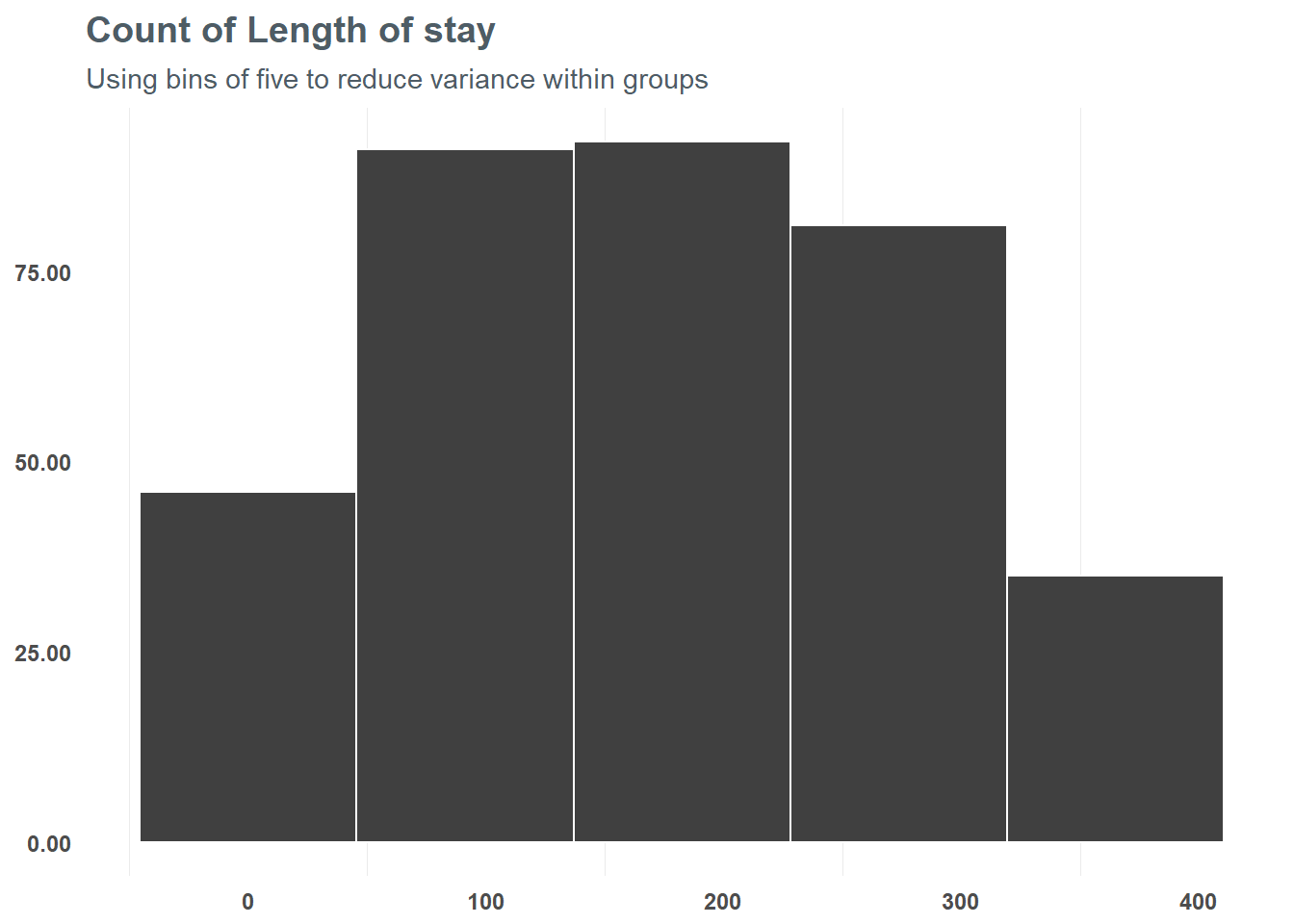
Creating dummy variables
I have a life-long goal of never using “one-hot-encoding” in an actual write-up, because I feel like “dummy variable” is a much better word and less fanciful. This process takes every single unique option of our categorical variables (again, variables like Gender and AnimalType) and creates individual variables for every option - and fills those variables with 1’s or 0’s denoting whether that condition exists or does not. For instance, for the Gender field we have variables like NEUTERED MALE. This process will create a new variable called NEUTERED MALE and register 1 whenever an animal is in fact a neutered male and a 0 whenever they are not. We do this process for every single character field - it will create a lot of new variables. Thankfully, we can process this with the recipes package - but it’s important to understand what we are doing.
Creating Our Recipe for Pre-Processing
First we prepare our recipe
A recipe is a step-by-step procedure for processing our data prior to modeling - just the same as baking a cake, we follow these steps to bake our model. Within these steps, we will create our bins for length_of_stay, log transform the age, create dummy variables for categorical variables, and center / scale our data to gain efficiency in the neural net model.
# Create recipe
train_recipe <- recipe(animal_euth ~ ., data = euth_train_tbl) %>%
  # Create 5 cuts of length_of_stay
  step_discretize(length_of_stay, options = list(cuts = 5)) %>%
  # Log transform age
  step_log(age) %>%
  # Generate dummy variables for all categoryical variables
  step_dummy(all_nominal(), -all_outcomes()) %>%
  # Center data
  step_center(all_predictors(), -all_outcomes()) %>%
  # Scale data
  step_scale(all_predictors(), -all_outcomes()) %>%
  # Prepare the recipe
  prep(data = euth_train_tbl)

# View the recipe
train_recipe
## Data Recipe
##
## Inputs:
##
## role #variables
## outcome 1
## predictor 12
##
## Training data contained 111049 data points and no missing data.
##
## Steps:
##
## Dummy variables from length_of_stay [trained]
## Log transformation on age [trained]
## Dummy variables from AnimalType, IntakeType, IntakeSubtype, ... [trained]
## Centering for age, AnimalType_CAT, ... [trained]
## Scaling for age, AnimalType_CAT, ... [trained]# Create recipe
test_recipe <- recipe(animal_euth ~ ., data = euth_test_tbl) %>%
# Create 5 cuts of length_of_stay
step_discretize(length_of_stay, options = list(cuts = 5)) %>%
# Log transform age
step_log(age) %>%
# Generate dummy variables for all categoryical variables
step_dummy(all_nominal(), -all_outcomes()) %>%
# Center data
step_center(all_predictors(), -all_outcomes()) %>%
# Scale data
step_scale(all_predictors(), -all_outcomes()) %>%
# Prepare the recipe
prep(data = euth_test_tbl)
# View the recipe
test_recipe## Data Recipe
##
## Inputs:
##
## role #variables
## outcome 1
## predictor 12
##
## Training data contained 27761 data points and no missing data.
##
## Steps:
##
## Dummy variables from length_of_stay [trained]
## Log transformation on age [trained]
## Dummy variables from AnimalType, IntakeType, IntakeSubtype, ... [trained]
## Centering for age, AnimalType_CAT, ... [trained]
## Scaling for age, AnimalType_CAT, ... [trained]Next we bake
Now that we have our recipe for pre-processing our data, we can apply that pre-processing (bake the recipe) against our training and test sets. Speaking from experience - this is insanely more efficient than the days of having to apply functions across your data. I wish this existed years ago!
# Set and process predictors
x_euth_train_tbl <- bake(train_recipe, newdata = euth_train_tbl)
x_euth_test_tbl  <- bake(test_recipe, newdata = euth_test_tbl)

# This isn't perfectly stratified, so remove columns from train that are not in test
x_euth_train_tbl <- x_euth_train_tbl[, which(names(x_euth_train_tbl) %in% names(x_euth_test_tbl))]

# Do the same with the test set
x_euth_test_tbl <- x_euth_test_tbl[, which(names(x_euth_test_tbl) %in% names(x_euth_train_tbl))]

# Take a look at the two dataframes
glimpse(x_euth_train_tbl[1:10])
## Observations: 111,049
## Variables: 10
## $ animal_euth <dbl> 0, 1, 1, 0, 1, 0, 0, 0, 0, 1, 0, 0, 0, 0,...
## $ age <dbl> 1.1653073, 0.6782845, -1.1944425, 0.85320...
## $ AnimalType_CAT <dbl> -0.941811, 1.061775, -0.941811, 1.061775,...
## $ AnimalType_DOG <dbl> 1.0088142, -0.9912538, 1.0088142, -0.9912...
## $ AnimalType_FERRET <dbl> -0.02382507, -0.02382507, -0.02382507, -0...
## $ AnimalType_LIVESTOCK <dbl> -0.042156, -0.042156, -0.042156, -0.04215...
## $ AnimalType_OTHER <dbl> -0.09685187, -0.09685187, -0.09685187, -0...
## $ AnimalType_RABBIT <dbl> -0.08896329, -0.08896329, -0.08896329, -0...
## $ AnimalType_REPTILE <dbl> -0.0441459, -0.0441459, -0.0441459, -0.04...
## $ AnimalType_RODENT <dbl> -0.06765621, -0.06765621, -0.06765621, -0...glimpse(x_euth_test_tbl[1:10])## Observations: 27,761
## Variables: 10
## $ animal_euth <dbl> 1, 1, 0, 1, 0, 0, 0, 1, 0, 1, 0, 1, 1, 0,...
## $ age <dbl> 0.8506475, -1.1963164, 0.5858991, 0.74551...
## $ AnimalType_CAT <dbl> -0.9421788, -0.9421788, -0.9421788, -0.94...
## $ AnimalType_DOG <dbl> 1.0105197, 1.0105197, 1.0105197, 1.010519...
## $ AnimalType_FERRET <dbl> -0.0287951, -0.0287951, -0.0287951, -0.02...
## $ AnimalType_LIVESTOCK <dbl> -0.0441463, -0.0441463, -0.0441463, -0.04...
## $ AnimalType_OTHER <dbl> -0.1002072, -0.1002072, -0.1002072, -0.10...
## $ AnimalType_RABBIT <dbl> -0.0873038, -0.0873038, -0.0873038, -0.08...
## $ AnimalType_REPTILE <dbl> -0.04029333, -0.04029333, -0.04029333, -0...
## $ AnimalType_RODENT <dbl> -0.06392924, -0.06392924, -0.06392924, -0...Capture target
In order to compare predictions to true data, we need to capture our training and test set target variable and store for comparison:
# Response variables for training and testing sets
y_euth_train_vec <- pull(euth_train_tbl, animal_euth)
y_euth_test_vec  <- pull(euth_test_tbl, animal_euth)
Run the Model
Now that we have our data processed and staged, we can build our Artificial Neural Network model. It seems like we did a lot just to finally get here, but typically that’s the case. The first 95% of the work done on a machine learning model is all data cleansing and processing - so we’re down to the final 5% - model building!
For some background, an ANN model is a multi-layered modeling approach designed to identify hidden interactions across individual variables that otherwise might go unseen. It’s extremely accurate as compared to more traditional modeling techniques, but also tends to be pretty “black box” in nature - so there is some tradeoff. Right now, I just want to get the thing running - once that happens, we can walk through ways to shed some light on the black box.
Initialize the model
Our first step is to initialize a sequential Keras model, and then add input/hidden/output layers to the sequential model.
The
input layeris the data itselfThe
hidden layersdefine the interactions between variables based on neural network nodes and the weights between them - there are alsodropout layerswhich are used to control for overfittingThe
output layerdefines the method of bringing all of the information together
# Building our Artificial Neural Network
keras_init <- keras_model_sequential()

keras_init %>%
    # First hidden layer
    layer_dense(
        units = 16,
        kernel_initializer = "uniform",
        activation = "relu",
        input_shape = ncol(x_euth_train_tbl)) %>%
    # Dropout to prevent overfitting
    layer_dropout(rate = 0.1) %>%
    # Second hidden layer
    layer_dense(
        units = 16,
        kernel_initializer = "uniform",
        activation = "relu") %>%
    # Dropout to prevent overfitting
    layer_dropout(rate = 0.1) %>%
    # Output layer
    layer_dense(
        units = 1,
        kernel_initializer = "uniform",
        activation = "sigmoid") %>%
    # Compile ANN
    compile(
        optimizer = 'adam',
        loss = 'binary_crossentropy',
        metrics = c('accuracy')
    )

keras_init
## Model
## ___________________________________________________________________________
## Layer (type) Output Shape Param #
## ===========================================================================
## dense_1 (Dense) (None, 16) 8112
## ___________________________________________________________________________
## dropout_1 (Dropout) (None, 16) 0
## ___________________________________________________________________________
## dense_2 (Dense) (None, 16) 272
## ___________________________________________________________________________
## dropout_2 (Dropout) (None, 16) 0
## ___________________________________________________________________________
## dense_3 (Dense) (None, 1) 17
## ===========================================================================
## Total params: 8,401
## Trainable params: 8,401
## Non-trainable params: 0
## ___________________________________________________________________________Run the model
Using the fit() function on our training data, we can define the number of batches we want to run and the number of training cycles (epochs). Within each epoch we define the number of batch samples per gradient update. A high batch size will decrease the error within each training cycle (epoch). We can also define validation splits to avoid overfitting among cycles.
We can then print out and plot the results of the model to help understand performance against the training set
# Print the final model results
fit_keras
## Trained on 77,734 samples, validated on 33,315 samples (batch_size=50, epochs=35)
## Final epoch (plot to see history):
## val_loss: 0.02092
## val_acc: 0.9976
## loss: 0.004225
## acc: 0.9989# Plot the training/validation history of our Keras model
plot(fit_keras) +
labs(title = "ANN Model Performance by Epoch",
subtitle = "Accuracy and loss each level out over time")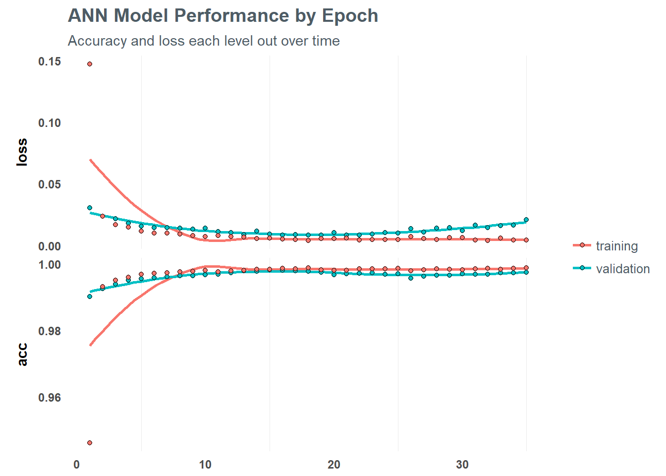
Making Predictions on Unseen Data
This is a really solid looking model - highly accurate within the training and validation sets. However - what about performance on unseen data? The model we ran against our training set may be dramatically underperforming on new data - which is why we sampled a separate chunk of data into a test set. We can apply the tuned ANN model to this test data, and see how well it performs.
# Create a vector of predictions
yhat_euth_vec <- predict_classes(object = keras_init, x = as.matrix(x_euth_test_tbl)) %>%
    as.vector()

# Create a vector of predicted probabilities of animal_euth = 1
yhat_euth_prob_vec  <- predict_proba(object = keras_init, x = as.matrix(x_euth_test_tbl)) %>%
    as.vector()
Compare prediction to actual
Now that we have our prediction on the held-out test data and we know the actuals, we can compare results and diagnose accuracy for our model. This is generally done through a combination of a confusion matrix (a 2x2 matrix of true/false predictions vs true/false actuals), and the area under the receiver operating charactersic (AUC, ROC) curve. This measures the True Positive Rate (TPR) vs. False Positive Rate (FPR) - and the area under is maximized when the model is not sacrificing Sensitivity (TPR) for Specificity (True Negative Rate).
So, let’s first look at the confusion matrix:
# Format prediction and actuals
estimates_euth_tbl <- tibble(
  truth = as.factor(y_euth_test_vec) %>% fct_recode(yes = "1", no = "0"),
  estimate = as.factor(yhat_euth_vec) %>% fct_recode(yes = "1", no = "0"),
  class_prob = yhat_euth_prob_vec %>% percent(2)
)

estimates_euth_tbl
## # A tibble: 27,761 x 3
## truth estimate class_prob
## <fctr> <fctr> <S3: formattable>
## 1 yes yes 100.00%
## 2 yes yes 100.00%
## 3 no no 0.00%
## 4 yes yes 100.00%
## 5 no no 0.00%
## 6 no no 0.00%
## 7 no no 0.00%
## 8 yes yes 100.00%
## 9 no no 0.00%
## 10 yes yes 100.00%
## # ... with 27,751 more rows# Create confusion table
estimates_euth_tbl %>% conf_mat(truth, estimate)## Truth
## Prediction no yes
## no 15110 10
## yes 49 12592The way to read the confusion matrix is:
For every animal predicted to be euthanized in our test set, 12,597 animals were in fact euthanized (these are true positives)
For every animal predicted to be euthanized, 44 actually were not (these are false positives)
For every animal not predicted to be euthanized, 15,090 animals were in fact not euthanized (these are true negatives)
For every animal not predicted ot be euthanized, 2 actually were euthanized (these are false negatives)
Walking through the numbers, the model seems to have performed pretty well. We can verify that further by calculating the area under the ROC curve - which is a barometer of how well calibrated the model is to the true positive rate and true negative rates (alluded to above). Essentially, the AUC tells us how balanced the model is at identifing animals as being euthanized at the expense of incorrectly identifying those that will not be euthanized.
In our case, the AUC for this model is 99.97%. Which is an extremely strong AUC! There are a couple of other tools to use to diagnose a model - such as the F1 score, which calculates a weighted average between the TPR and model’s recall (the number of correct positive predictions). In our model, our F1 score comes out to 99.81% - again, an extremely well tuned model it seems.
Lifting the Black Box
Now, this is all well and good and in theory we can apply this model on new data to predict the risk of any given animal at LMAS to be euthanized - but it doesn’t help identify the risk factors to shed light on. To do that, we can use a couple of tools - most accessible being a correlation plot from the corrr package.
Correlation plots show us individual relationships between each input variable and the target variable. This also stands as a good gut check to the feature importance (which, while not explicitly shown in this post, only age shows value when looking at feature importance on select observations).
# Feature correlations to euthanasia
corrr_analysis <- x_euth_train_tbl %>%
    mutate(animal_euth = y_euth_train_vec) %>%
    correlate() %>%
    focus(animal_euth) %>%
    rename(feature = rowname) %>%
    arrange(abs(animal_euth)) %>%
    mutate(feature = as_factor(feature))

corrr_analysis %>% arrange(desc(animal_euth))
## # A tibble: 505 x 2
## feature animal_euth
## <fctr> <dbl>
## 1 ReproductiveStatusAtIntake_UNKNOWN 0.2488139
## 2 Gender_UNKNOWN 0.2438192
## 3 Gender_MALE 0.2024663
## 4 AnimalType_CAT 0.2000811
## 5 PrimaryBreed_DOMESTIC.SHORTHAIR 0.1990997
## 6 IntakeReason_unknown 0.1661630
## 7 length_of_stay_bin3 0.1621148
## 8 IntakeAsilomarStatus_UNHEALTHY.UNTREATABLE 0.1365919
## 9 IntakeInternalStatus_SICK 0.1363610
## 10 IntakeInternalStatus_FERAL 0.0970065
## # ... with 495 more rowsInterestingly, when we look at the global relationships through correlation analysis we find that ReproductiveStatusAtIntake_UNKNOWN comes through as fairly significant positively, while age maintains a strong negative relationship. We can also visualize this information to show the differences.
# Correlation visualization
corr_plot <- corrr_analysis %>%
  ggplot(aes(x = animal_euth, y = fct_reorder(feature, desc(animal_euth)))) +
  geom_point() +
  # Positive Correlations - Contribute to churn
  geom_segment(aes(xend = 0, yend = feature),
               color = "#FF2C00",
               data = corrr_analysis %>% filter(animal_euth > 0)) +
    geom_point_interactive(color = "#FF2C00",
                           data = corrr_analysis %>% filter(animal_euth > 0),
                           aes(tooltip = paste0(
                             "<br><b> Feature: </b>",
                             feature,
                             "<br><b> Correlation: </b>",
                             animal_euth %>% percent(0)
                             ),
                             data_id = paste0(
                             "<br><b> Feature: </b>",
                             feature,
                             "<br><b> Correlation: </b>",
                             animal_euth %>% percent(0)
                             )
                             )) +
    # Negative Correlations - Prevent churn
    geom_segment(aes(xend = 0, yend = feature),
                 color = "#00AEF0",
                 data = corrr_analysis %>% filter(animal_euth < 0)) +
    geom_point_interactive(color = "#00AEF0",
                           data = corrr_analysis %>% filter(animal_euth < 0),
                           aes(tooltip = paste0(
                             "<br><b> Feature: </b>",
                             feature,
                             "<br><b> Correlation: </b>",
                             animal_euth %>% percent(0)
                             ),
                             data_id = paste0(
                             "<br><b> Feature: </b>",
                             feature,
                             "<br><b> Correlation: </b>",
                             animal_euth %>% percent(0)
                             )
                             )) +
    # Vertical lines
    geom_vline(xintercept = 0, color = "#A6A5A5", size = 1, linetype = 2) +
    geom_vline(xintercept = -0.25, color = "#A6A5A5", size = 0.75, linetype = 2) +
    geom_vline(xintercept = 0.25, color = "#A6A5A5", size = 0.75, linetype = 2) +
    # Aesthetics
    labs(title = "Animal Euthanasia Correlation Analysis",
         subtitle = "Positive Correlations (contribute to euthanasia), \nNegative Correlations (prevent euthanasia)",
         y = "Feature",
         x = "Correlation") +
  theme(axis.text.y = element_blank(),
        axis.ticks = element_blank())

ggiraph(code = print(corr_plot),
        width = 1,
        height = 6,
        hover_css = "cursor:pointer;fill:#ff8500;stroke:#ff8500;")
With over 500 variables to test, this is a bit messy to look at. So let’s limit down to just those variables with either less than -0.25 or greater than 0.25 correlation. At that point, it’s a flip of a coin whether a given feature is influencing the variation in euthanasias.
# Correlation visualization
corr_significant <- corrr_analysis %>%
  filter(animal_euth > 0.10 | animal_euth < -0.10)

corr_plot_significant <- corr_significant %>%
  ggplot(aes(x = animal_euth, y = reorder(feature, -animal_euth))) +
  geom_point() +
  # Positive Correlations - Contribute to churn
  geom_segment(aes(xend = 0, yend = feature),
               color = "#FF2C00",
               data = corr_significant %>% filter(animal_euth > 0)) +
    geom_point_interactive(color = "#FF2C00",
                           data = corr_significant %>% filter(animal_euth > 0),
                           aes(tooltip = paste0(
                             "<br><b> Feature: </b>",
                             feature,
                             "<br><b> Correlation: </b>",
                             animal_euth %>% percent(0)
                             ),
                             data_id = paste0(
                             "<br><b> Feature: </b>",
                             feature,
                             "<br><b> Correlation: </b>",
                             animal_euth %>% percent(0)
                             )
                             )) +
    # Negative Correlations - Prevent churn
    geom_segment(aes(xend = 0, yend = feature),
                 color = "#00AEF0",
                 data = corr_significant %>% filter(animal_euth < 0)) +
    geom_point_interactive(color = "#00AEF0",
                           data = corr_significant %>% filter(animal_euth < 0),
                           aes(tooltip = paste0(
                             "<br><b> Feature: </b>",
                             feature,
                             "<br><b> Correlation: </b>",
                             animal_euth %>% percent(0)
                             ),
                             data_id = paste0(
                             "<br><b> Feature: </b>",
                             feature,
                             "<br><b> Correlation: </b>",
                             animal_euth %>% percent(0)
                             )
                             )) +
    # Vertical lines
    geom_vline(xintercept = 0, color = "#A6A5A5", size = 1, linetype = 2) +
    geom_vline(xintercept = -0.10, color = "#A6A5A5", size = 0.5, linetype = 2) +
    geom_vline(xintercept = 0.10, color = "#A6A5A5", size = 0.5, linetype = 2) +
    geom_vline(xintercept = -0.25, color = "#A6A5A5", size = 0.75, linetype = 2) +
    geom_vline(xintercept = 0.25, color = "#A6A5A5", size = 0.75, linetype = 2) +
    # Aesthetics
    labs(title = "Most Significant Features to Euthanasia",
         subtitle = "Positive Correlations (contribute to euthanasia), \nNegative Correlations (prevent euthanasia)",
         y = "",
         x = "Correlation") +
  theme(axis.ticks = element_blank(),
        axis.text = element_text(size = 6))

ggiraph(code = print(corr_plot_significant),
        width = 1,
        height = 6,
        hover_css = "cursor:pointer;fill:#ff8500;stroke:#ff8500;")
This lets us see a little more clearly what factors weigh most heavily on the odds of an animal being euthanized. We can see that animals with very little known history (unknown reproductive status, unknown gender, unknown intake reason) seems to increase the odds an animal is euthanized. On the flip side, age and whether an animal is neutered or spayed tend to lower the odds. In addition, animals returned or fostered tend to make it out better than not.
The age variable is pretty interesting - particularly when we break it down. When looking at feature importance, younger age buckets tend to have a greater level of importance in predicting whether an animal will be euthanized. That conclusion seems to be supported in the correlation analysis - as the negative correlation means an increase in age implies a decrease in likelihood (although, this is a pretty big generalization and the shape of that relationship may be different in later years).
What Can I Do With This Information?
While this has been an extremely effective way for me to learn new tools and modeling techniques, there is a larger purpose involved as well - as mentioned at the beginning. Ultimately, I wanted to use this work to understand which animals at LMAS have the highest probability for being euthanized. This way I can try and highlight these animals for others who are considering adopting, including my own family.
To do this, we can build a table of animals who are considered high-risk in my model and are still at LMAS (as of 2017-12-02). This table below shows all animals that are currently within the LMAS system - as well as their breed, age, and current length of stay. If you are interested in learning more about any of these animals, you can click on the Animal ID and the link will take you to their page at petharbor.com. Please consider looking at these animals - they all deserve great homes!
Next Steps
This project was ultimately a great opportunity for me to learn several new tools while also helping me to research a topic that I am passionate about. In no way should the list above be considered “official” in terms of what animals will or will not be euthanized by LMAS. The organization has done an amazing job at reducing the kill rate at their shelter (as evidenced in the chart at the beginning) - but I hope this analysis will help move folks toward adoption that are considering bringing a new family member into their home.
That said, I want to highlight some “next steps” I am considering before some of the data nerds out there call me out:
Data Limitations
First, I would like to point out that the data we are working with here is not perfect by any means. The system of collection is not necessarily set up for this type of analysis - and therefore, I would need to spend more time on clean up to get it closer to perfect. There are a couple of areas I am most interested in from a feature engineering standpoint:
Multiple Visits
Some of these animals are frequent visitors at LMAS. It wouldn’t be difficult to make this a separate input feature, but honestly I got lazy there. I will be adding this for an update to this - so stay tuned!
Temporal Differences
As mentioned earlier, the rate of euthanasia is decreasing over time. Because of this, it’s not exactly perfect to use a generalized model built over several years to this year. That said, any bias would be generalized across the board most likely as it seems to be a population trend and not over represented within any specific groups of animals. Because of this, the conclusion of which animals are most at risk still largely stands. The only difference would be that their individual odds may be lower across the board.
Model Limitations
In the interest of time, I didn’t tweak much of what was already done in the original Business-Science article. This was mostly because I used this as an opportunity to learn ANN and keras, but also because I wanted to get a fairly well-tuned model out and I am sort of piggybacking on those guys having done the work ahead of time for me to pick some of the right hyperparameters (batch sizes, kernels, etc.). In future updates, I will tune those hyperparameters for this analysis.
Conclusion
Ultimately, I am satisfied with what the results are showing. There are obviously limitations here - but with some more time dedicated, they are fixable and I do not believe they will dramatically shift the outcome. Measured against eachother, the list of animals in the table above represents those that pose the highest risk of euthanasia from my ANN model. Luckily, LMAS has done a tremendous job at pushing the overall rate of euthanasia lower, but they are not able to save every animal – so please, consider adopting (and consider adopting an animal from that list). The more we adopt, the more LMAS can save!