Background

The purpose of this tutorial is to walk through using d3.js within an Rmd document that is then rendered as an HTML page with a Hugo static site generator. That was probably the most technical sentence of this entire write-up, so let’s all breath a sigh of relief now that we’re through with it.

This is a quick release, so I’m not going to go into much detail about the process to get the data and what it fully represents just yet - I’m saving that for a deeper post with a “tbd” release date at this point. Just trust that the data is legit for now, and reach out if you want a pre-release introduction to it all.

Setup

There are a couple of things that I am going to assume:

1. You have a Hugo site setup already
2. You’re at least comfortable with d3 and knitr code chunks
3. You know the basics of Rmarkdown

If you’re cool with those three things, then you should be able to follow along and will probably already know more than I did when I first learned how to do this. If you aren’t too familiar with them, the keep reading! This is written from the context of having just learned how to do it myself - and hopefully it will be somewhat interesting still!

Staging the data

As is always the case when it comes to data analysis, the most important piece of the puzzle here is the data. In particular, how we stage the data for the d3 visualization is extremely important. Just about everything done in R is done using data in a nice and tidy rectangular format - meaning your rows are observations and your columns are variables. This makes it easy to do math-y things, but just about everything else in the world likes data to be a bit more nested. This is the case for d3 - which works based with JSON files when building out visualizations.

For instance, the data we are working with is a dataframe that is 4 columns wide by 900 rows long, and looks pretty clean:

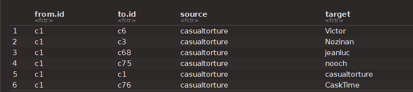
If we were building some kind of weird statistical model off of this data, we would be set. But we’re not, so we aren’t - and instead we need to get the data setup in the preferred JSON format before we can build our d3 object. To take care of that, we can use jsonlite::toJSON to handle the conversion, and create a <script>...</script> HTML element at the same time so that we can pass the data object to d3.

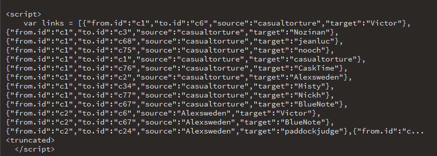
For example, the following chunk will take our rectangular dataframe edges_expanded and transform it into a JSON file that is assigned to the variable name links. It is crucial that when doing this, you pass through results="asis" and that you do not set include = FALSE. Otherwise, the data will not be passed to the d3 element, and your whole day will be ruined.

# Build <script>...</script> element to pass data to d3 as 'links' variable
cat(
  paste(
  '<script>
    var links = ',toJSON(edges_expanded),';
  </script>'
  , sep="")
)

The result of this is not quite as pretty, but you can see that the paste function is essentially building out a <script> HTML element that creates the links variable for us. Nifty trick! At this point, our data is setup and ready to go for a d3 visualization.

Building the visual

At this point, we have our data staged in the right format and we’ve built our <script> element to pass the links variable through. All that is left now is to build out our d3 element within our Rmarkdown document, and then we can let Hugo do the rest for us!

Building the d3 element is deceptively easy - especially if you already have the pieces put together separately. In fact, by keeping the data and visualization all in one place (in this case, building everything within RStudio), embedding a d3 element into an Rmarkdown file is (in my opinion, at least) way easier than trying to develop it into a raw HTML object.

To do so, you simply set a new div element - in this case, we are giving it the ID “plot” - and then append your SVG element to that div.

<script src="https://d3js.org/d3.v3.min.js"></script>

<script>

var width = 950,
    height = 700;

var svg = d3.select("#plot").append("svg")
    .attr("width", width)
    .attr("height", height);

That will give us the basic structure of our SVG element that we will then layer our data onto. I’m not going to get into how to set the force layout we are using here, but to build out our nodes (the user-defined circles) we can use the following:

// Create nodes for each unique source and target.
links.forEach(function(link) {
  link.source = nodeByName(link.source);
  link.target = nodeByName(link.target);
});

The chunk takes our pre-defined variable links and assigns two new objects: link.source and link.target. These are used throughout the d3 layout to build the source and target nodes - essentially telling the object how to (uh, literally) connect the dots.

From there, we can build line elements between the link objects, and also layer over some of the fancy mouseover functionality to show username or connected nodes. As mentioned, I’m not going to get into those details - but the passing of data from a code chunk to a d3 element in Rmarkdown is extremely useful.

Pushing the blog post

If you’ve made it this far, then you’re pretty much done. Simply run the function blogdown::build_site() and Hugo handles the rest. If you are publishing your /public content to your host server then you should see your post update and render your d3 visualization at this point. Or, if you are using the two-repo method w/ github pages - once you push the changes in /public to your github.io repo you should be good to go!